The Linear Mixed Models Toolbox
Introduction
The Linear mixed Models Toolbox (lmt) is a stand-alone single executable software for for large scale linear mixed model analysis. It is the successor of DMU, the well-known and widely used software package for linear mixed model analysis developed and maintained by Per Madsen and Just Jensen.
Since the early days of software development in statistics and quantitative genetics time has moved on in terms of what programming languages are capable of and therefore DMU has been given a thorough overhaul.
One result of the overhaul is the new name, lmt, resulting from the difficulty to translate the acronym DMU into something which is generally meaningful throughout time. For those who prefer the acronym DMU, they may refer to lmt as DMU-next.
The second area of the overhaul is the parameter file interface. lmt now comes with an xml style parameter file which is supposed to allow for a much easier understanding by the user. Further using xml comes with support for automated commenting, un- commenting, indentation, code-folding and syntax highlighting by almost every editor, thus easing to follow the structure of the parameter file even if it spans several tens of lines of code.
The third area of the overhaul is the program structure. DMU was structured into several programs (DMU1, DMU4, DMU5, DMUAI, RJMC). In contrast, lmt is meant to provide the functionalities all those programs via a single parameter file and a single executable.
While lmt is finally meant to be a full scale successor of DMU, it does not yet provide all its functionalities in some areas, in others it already provides more. More specifi- cally, there no REML facilities available yet, but large scale linear mixed model solving provides Single-Step-T-BLUP facilities, uploading of genotypes and building of genomic relationship matrices on the fly etc etc.
Supported features
Supported operations
Currently lmt support the following operations on linear mixed models:
- Solving for BLUP and BLUE solutions conditional on supplied variances for random and fixed factor, respectively;
- Gibbs sampling of variance components in single pass and blocked mode;
- MC-EM-REML estimation of variance components
- Sampling elements of the inverse of the mixed model coefficient matrix
Supported factors and variables
lmt supports
- fixed
- random factors
- classification variables
- continuous co-variables, which can be nested. For continuous co-variables lmt support user-defined polynomials and hard coded Legendre polynomials up to order 6.
- genetic group co-variables
All classification and co-variables can be associated to a fixed or random factor.
Supported variance structures
For random factor lmt supports variance structures of
- structure $$\Gamma\otimes\Sigma$$, where $$\Sigma$$ is an dense symmetric positive definite matrix, and
- $$\Theta_L(\Gamma\otimes I_{\Sigma})\Theta_L^{'}$$, where $$\Theta$$ is symmetric positive definite block-diagonal matrix of $$n$$ symmetric positive definite martices $$\Sigma_i, i=1,..,n$$, $$\Theta_L$$ is the lower Cholesky factor of $$\Theta$$ and $$I_{\Sigma}$$ is an identity matrix of dimension $$\Sigma_i$$.
When solving linear mixed models $$\Sigma$$ and $$\Gamma$$ are user determined constants, whereas when estimating variances $$\Gamma$$ is a user determined constant and $$\Sigma$$ is a function of the data.
Supported type for $$\Gamma$$ are
- an identity matrix
- an arbitrary positive definite diagonal matrix
- a pedigree-based numerator relationship matrix $$A$$ which may contain meta-founders
- a pedigree- and genotype-based relationship matrix $$H$$ which may contain meta-founders
- a user-defined(u.d.) symmetric, positive definite matrix of which inverse is supplied
- as a sparse upper-triangular matrix stored in csr format
- as a dense matrix
- a co-variance matrix of a selected auto-regressive process
Supported linear mixed model solvers
lmt supports
- a direct solver requiring to explicitly build the linear mixed model equations left-hand-side coefficient matrix($$C$$)
- an iteration-on-data pre-conditioned gradient solver which does not require $$C$$
- direct use of genomic marker data
- building of genomic relationship matrices($$G$$) from supplied genomic data
- uploading of a u.d. $$G$$
- adjustment of $$G$$ to $$A_{gg}$$
- solving Single-Step-G-BLUP models
- sampling variances for Single-Step-G-BLUP models
- solving Single-Step-T-BLUP models
- solving Single-Step-SNP-BLUP models
- all Single-Step models can be run from "bottom-up", that is the user supplies the genotypes and all necessary ingredients(e.g. $$G$$) are built on the fly.
Supported pedigree types
- ordinary pedigrees
- probabilistic pedigrees with an unlimited number of parent pairs per individual
- genetic group pedigrees
- meta-founders
lmt Linear mixed model terminology
Matrix notation, factors and sub-factors
Consider the multi-variate linear mixed model
$$ \left( \begin{array}{c} y_1 \\ y_2 \\ y_3 \end{array} \right) = \left( \begin{array}{ccc} X_1 & 0 & 0 \\ 0 & X_2 & 0 \\ 0 & 0 & X_3 \end{array} \right) \left( \begin{array}{c} b_1 \\ b_2 \\ b_3 \end{array} \right) + \left( \begin{array}{ccc} Z_1 & 0 & 0\\ 0 & Z_2 & 0\\ 0 & 0 & Z_3 \end{array} \right) \left( \begin{array}{c} u_1 \\ u_2 \\ u_3 \end{array} \right) + \left( \begin{array}{c} e_1 \\ e_2 \\ e_3 \end{array} \right) $$
where $$(y_1,y_2,y_3)'$$, $$(b_1,b_2,b_3)'$$, $$(u_1,u_2,u_3)'$$ and $$(e_1,e_2,e_3)'$$ are vectors of response variables, effects of fixed factors, effects of random factors and effects of residuals respectively, and matrices $$\left( \begin{array}{ccc} X_1 & 0 & 0 \\ 0 & X_2 & 0 \\ 0 & 0 & X_3 \end{array} \right)$$, and $$ \left( \begin{array}{ccc} Z_1 & 0 & 0\\ 0 & Z_2 & 0\\ 0 & 0 & Z_3 \end{array} \right) $$ are block-diagonal design matrices linking effects in the respective vectors to their related response variables. In usual mixed model terminology $$b_1$$, $$b_2$$ and $$b_3$$ are called fixed factors, and $$u_1$$, $$u_2$$ and $$u_3$$ are called random factors. Ignoring the residual the above model has in total 6 factors.
However, the model maybe rewritten in matrix formulation as
$$vec(Y)=Xvec(B)+Zvec(U)+vec(E)$$,
where $$vec$$ is the vectorization operator, $$Y=[y_1,y_2,y_3]$$, $$B=[b_1,b_2,b_3]$$, $$U=[u_1,u_2,u_3]$$ and $$E=[e_1,e_2,e_3]$$ are column matrices of response variables, the effects of the fixed and random factor, and the residuals, respectively, and $$X=\left( \begin{array}{ccc} X_1 & 0 & 0 \\ 0 & X_2 & 0 \\ 0 & 0 & X_3 \end{array} \right)$$, and $$Z= \left( \begin{array}{ccc} Z_1 & 0 & 0\\ 0 & Z_2 & 0\\ 0 & 0 & Z_3 \end{array} \right) $$. The distribution assumption for the random components in the model are $$vec(U^{'})\sim N((0,0,0)',\Gamma_u \otimes \Sigma_u)$$ and $$vec(E^{'})\sim N((0,0,0)',\Gamma_e \otimes \Sigma_e)$$. Note that the column and row dimensions of $$U$$ are determined by the column dimension of $$\Sigma_u$$ and $$\Gamma_u$$ respectively.
Slightly different to the above terminology, lmt refers to $$B$$ and $$U$$ as factors, and therefore the model has only two factors, whereas the columns in $$B$$ and $$U$$ are referred to as sub-factors.
Following the above matrix notation lmt will always invoke only one factor for all modelled fixed classification variables and only one factor for all modelled fixed continuous co-variables. Sub-factors are summarized into a single random factors if they share the same $$\Sigma$$ matrix. Thus, lmt will invoke as many random factors as there are different $$\Gamma \otimes \Sigma$$ constructs. That is, in lmt terminology the multi-variate model
$$ \left( \begin{array}{c} y_1 \\ y_2 \\ y_3 \end{array} \right) = \left( \begin{array}{ccc} X_1 & 0 & 0 \\ 0 & X_2 & 0 \\ 0 & 0 & X_3 \end{array} \right) \left( \begin{array}{c} b_1 \\ b_2 \\ b_3 \end{array} \right) + \left( \begin{array}{cccccc} Z_{d,1} & 0 & 0 & Z_{m,1} & 0 & 0\\ 0 & Z_{d,2} & 0 & 0 & Z_{m,2} & 0\\ 0 & 0 & Z_{d,3} & 0 & 0 & Z_{m,3}\\ \end{array} \right) \left( \begin{array}{c} u_{d,1} \\ u_{d,2} \\ u_{d,3} \\ u_{m,1} \\ u_{m,2} \\ u_{m,3} \end{array} \right) + \left( \begin{array}{ccc} W_1 & 0 & 0\\ 0 & W_2 & 0\\ 0 & 0 & W_3 \end{array} \right) \left( \begin{array}{c} v_1 \\ v_2 \\ v_3 \end{array} \right) + \left( \begin{array}{c} e_1 \\ e_2 \\ e_3 \end{array} \right) $$
with $$(u_{d,1},u_{d,2},u_{d,3},u_{m,1},u_{m,2},u_{m,3})'\sim N((0,0,0,0,0,0)',\Sigma_u \otimes \Gamma_u)$$ and $$(v_1,v_2,v_3)'\sim N((0,0,0)',\Sigma_v \otimes \Gamma_v)$$, rewritten as $$vec(Y)=Xvec(B)+Zvec(U)+Wvec(V)+vec(E)$$ will have only 3 factors, $$B$$, $$U$$ and $$V$$ with $$b_1,b_2,b_3$$, $$u_{d,1},u_{d,2},u_{d,3},u_{m,1},u_{m,2},u_{m,3}$$ and $$v_1,v_2,v_3$$ being subfactors of $$U$$ and $$V$$ respectively.
Model syntax
The syntax for communicating the model to lmt is effectively just write the model.
A valid lmt model string would y=mu*b+id*u(v(my_var(1))) . The model string consist of
- the response variable y , which must be a column name in the data file
- variables mu and id , which must be a column names in the data file
- sub-factors b and u which are user-defined alpha-numeric character strings
- relation operators = , * and +
- a specifier (v(my_var(1))) used to specify the nature of u
The rules for using relational operators are
- = links the response variable to the model
- * links a model variable to it's sub-factor, which together form a right hand side component
- + concatenates different right hand side components.
Specifiers
Variables and sub-factors maybe accompanied by a specifier. A specifier is a tree diagramm in Newick format with all nodes named, but leaf nodes can be unnamed, and where the root node name is the variable or sub-factor name. The specifier provides additional information about a variable or sub-factor. The lmt version of the above tree diagram differs in that
- the parent nodes precede child nodes
- child nodes within the same parent node are separated by semicolon
- sibling nodes can be mutually exclusive, that is only one sibling node maybe allowed
- leaf nodes maybe not named but contain additional, maybe comma-separated information
- if a child node is marked as default, the child node and it's immediate parent node can be omitted
- if a node is marked as optional it can be omitted. if an optional node is used it's compulsory child nodes must be included
Variable specifiers
Variable specifiers are used to communicate further information which may be that the variable
- is continuous but real numbers
- is continuous but integer numbers
- is a genetic group regression matrix
- undergoes a polynomial expansion
- is associated to a nesting variable
etc.
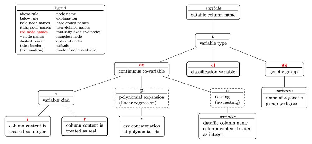
The tree diagram for the variable specifier is
with the nested parentheses representation written as
variable(t(co(t(i;r);p(polynomial ids);n(variable));cl;gg(pedigree)))
Note that the above representation would not yield a valid specifier useable in an equation as the diagram contains sibling nodes which are mutually exclusive, thus allowing only one of the sibling node to occur in the specifier. That is valid specifiers would be
variable(t(cl))
variable(t(gg(pedigree)))
variable(t(co(t(i);p(polynomial id);n(variable))))
variable(t(co(t(i);p(polynomial id);n(variable))))
Since a default-determining leave node and it's immediate parent node can be omitted the following equality holds:
variable(t(cl))=variable
Sub-factor specifiers
Sub-factor specifiers are used to communicate further information which may be that the sub-factor
- is a random sub-factor
- to which variance it is related to
- which diagonal element in the $$\Sigma$$ matrix of the variance it is related to
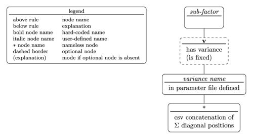
The tree diagram for the sub-factor specifier is
with the nested parentheses representation written as
sub-factor(v(variance name(diagonal position)))
According to the tree diagram the sub-factor specifier in the example model string in #Model syntax translates to
- sub-factor name is u
- the sub-factor has a variance
- variance name is my_var
- the diagonal position in $$\Sigma$$ is #1.
Variables as well as sub-factors maybe used across traits. That is a model
y1=mu*b1+id*u1(v(sigma(1))
y2=mu*b2+id*u2(v(sigma(2))
Disclaimer
lmt is under ongoing development and many of its features have been tested only a few times on a limited number of models and data sets. Thus, the users uses lmt completely on his/her own risk. This also applies to any decisions made based on the results provided by lmt.
Conditions of use
lmt can be used by the scientific community free of charge, but users must credit lmt in any publications. Commercial users must obtain the explicit approval of the author before using lmt and must credit lmt in any publication in scientific journals.
Feedback and support
lmt comes without any guaranteed support and the user is strongly advised to study the manual thoroughly. However, the author appreciates feedback about the program functionality, possible aborts (segmentation faults), usability of output and comprehensiveness of the manual.

