Linear mixed models in lmt

Matrix notation, factors and sub-factors

Consider the multi-variate linear mixed model

$$ \left( \begin{array}{c} y_1 \\ y_2 \\ y_3 \end{array} \right) = \left( \begin{array}{ccc} X_1 & 0 & 0 \\ 0 & X_2 & 0 \\ 0 & 0 & X_3 \end{array} \right) \left( \begin{array}{c} b_1 \\ b_2 \\ b_3 \end{array} \right) + \left( \begin{array}{ccc} Z_1 & 0 & 0\\ 0 & Z_2 & 0\\ 0 & 0 & Z_3 \end{array} \right) \left( \begin{array}{c} u_1 \\ u_2 \\ u_3 \end{array} \right) + \left( \begin{array}{c} e_1 \\ e_2 \\ e_3 \end{array} \right) $$

where $$(y_1,y_2,y_3)'$$, $$(b_1,b_2,b_3)'$$, $$(u_1,u_2,u_3)'$$ and $$(e_1,e_2,e_3)'$$ are vectors of response variables, effects of fixed factors, effects of random factors and effects of residuals respectively, and matrices $$\left( \begin{array}{ccc} X_1 & 0 & 0 \\ 0 & X_2 & 0 \\ 0 & 0 & X_3 \end{array} \right)$$, and $$ \left( \begin{array}{ccc} Z_1 & 0 & 0\\ 0 & Z_2 & 0\\ 0 & 0 & Z_3 \end{array} \right) $$ are block-diagonal design matrices linking effects in the respective vectors to their related response variables. In usual mixed model terminology $$b_1$$, $$b_2$$ and $$b_3$$ are called fixed factors, and $$u_1$$, $$u_2$$ and $$u_3$$ are called random factors. Ignoring the residual the above model has in total 6 factors.

However, the model maybe rewritten in matrix formulation as

$$vec(Y)=Xvec(B)+Zvec(U)+vec(E)$$,

where $$vec$$ is the vectorization operator, $$Y=[y_1,y_2,y_3]$$, $$B=[b_1,b_2,b_3]$$, $$U=[u_1,u_2,u_3]$$ and $$E=[e_1,e_2,e_3]$$ are column matrices of response variables, the effects of the fixed and random factor, and the residuals, respectively, and $$X=\left( \begin{array}{ccc} X_1 & 0 & 0 \\ 0 & X_2 & 0 \\ 0 & 0 & X_3 \end{array} \right)$$, and $$Z= \left( \begin{array}{ccc} Z_1 & 0 & 0\\ 0 & Z_2 & 0\\ 0 & 0 & Z_3 \end{array} \right) $$. The distribution assumption for the random components in the model are $$vec(U^{'})\sim N((0,0,0)',\Gamma_u \otimes \Sigma_u)$$ and $$vec(E^{'})\sim N((0,0,0)',\Gamma_e \otimes \Sigma_e)$$. Note that the column and row dimensions of $$U$$ are determined by the column dimension of $$\Sigma_u$$ and $$\Gamma_u$$ respectively.

Slightly different to the above terminology, lmt refers to $$B$$ and $$U$$ as factors, and therefore the model has only two factors, whereas the columns in $$B$$ and $$U$$ are referred to as sub-factors.

Following the above matrix notation lmt will always invoke only one factor for all modelled fixed classification variables and only one factor for all modelled fixed continuous co-variables. Sub-factors are summarized into a single random factors if they share the same $$\Sigma$$ matrix. Thus, lmt will invoke as many random factors as there are different $$\Gamma \otimes \Sigma$$ constructs. That is, in lmt terminology the multi-variate model

$$ \left( \begin{array}{c} y_1 \\ y_2 \\ y_3 \end{array} \right) = \left( \begin{array}{ccc} X_1 & 0 & 0 \\ 0 & X_2 & 0 \\ 0 & 0 & X_3 \end{array} \right) \left( \begin{array}{c} b_1 \\ b_2 \\ b_3 \end{array} \right) + \left( \begin{array}{cccccc} Z_{d,1} & 0 & 0 & Z_{m,1} & 0 & 0\\ 0 & Z_{d,2} & 0 & 0 & Z_{m,2} & 0\\ 0 & 0 & Z_{d,3} & 0 & 0 & Z_{m,3}\\ \end{array} \right) \left( \begin{array}{c} u_{d,1} \\ u_{d,2} \\ u_{d,3} \\ u_{m,1} \\ u_{m,2} \\ u_{m,3} \end{array} \right) + \left( \begin{array}{ccc} W_1 & 0 & 0\\ 0 & W_2 & 0\\ 0 & 0 & W_3 \end{array} \right) \left( \begin{array}{c} v_1 \\ v_2 \\ v_3 \end{array} \right) + \left( \begin{array}{c} e_1 \\ e_2 \\ e_3 \end{array} \right) $$

with $$(u_{d,1},u_{d,2},u_{d,3},u_{m,1},u_{m,2},u_{m,3})'\sim N((0,0,0,0,0,0)',\Sigma_u \otimes \Gamma_u)$$ and $$(v_1,v_2,v_3)'\sim N((0,0,0)',\Sigma_v \otimes \Gamma_v)$$, rewritten as $$vec(Y)=Xvec(B)+Zvec(U)+Wvec(V)+vec(E)$$ will have only 3 factors, $$B$$, $$U$$ and $$V$$ with $$b_1,b_2,b_3$$, $$u_{d,1},u_{d,2},u_{d,3},u_{m,1},u_{m,2},u_{m,3}$$ and $$v_1,v_2,v_3$$ being subfactors of $$U$$ and $$V$$ respectively.

Model syntax

The syntax for communicating the model to lmt is effectively: "just write the model", where the model is written into the space of a particular xml element of the parameter file.

Note that lmt will only check whether the specified model can be built, not whether the model is meaningful or allows for a statistical inference.

An example

An example for a valid lmt model string would be

y=x*b+age(t(co(p(1,2))))*c+id*u(v(my_var(1))).

The components of the model string are

• the response variable y , which must be a column name in the data file
• model variables x , age and id , which must be a column names in the data file
• sub-factors b , c and u which are user-defined alpha-numeric character strings
• relation operators = , * and +
• a variable specifier (t(co(p(1,2)))) used to provide further information about variable age
• a sub-factor specifier (v(my_var(1))) used to provide further information about sub-factor u

Variables

Response variables and model variables are named using user-defined alpha-numeric character strings. These character strings must be column names in the data file. There is no size limitation for the variables names.

Model variables can be used in several equations. That is, the bi-variate model

y1=x*b1
y2=x*b2,

with variables x, y1 and y2 being column names in the data file, is equivalent to the model $$ \left( \begin{array}{c} y_1 \\ y_2 \end{array} \right)= \left( \begin{array}{cc} X & 0 \\ 0 & X \end{array} \right) \left( \begin{array}{c} b_1 \\ b_2 \end{array} \right)+ \left( \begin{array}{c} e_1 \\ e_2 \end{array} \right) $$

Sub-factors

Sub-factors are named using user-defined alpha-numeric character strings. There is no size limitation for the variables names.

Contrarily to using variables across traits, using a sub-factor across traits changes the model. That is model

y1=x*b1
y2=x*b1

is equivalent to $$ \left( \begin{array}{c} y_1 \\ y_2 \end{array} \right)= \left( \begin{array}{c} X \\ X \end{array} \right) \begin{array}{c} b_1 \\ \end{array} + \left( \begin{array}{c} e_1 \\ e_2 \end{array} \right) $$

Relational operators

The rules for using relational operators are

• = links a single response variable to the model
• * links a model variable to it's sub-factor, which together form a model term
• + concatenates different model terms.

Specifiers

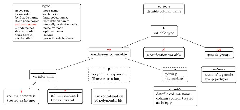
Variables and sub-factors maybe accompanied by a specifier. A specifier is a tree diagramm in Newick format with all nodes named, but leaf nodes can be unnamed, and where the root node name is the variable or sub-factor name. The specifier provides additional information about a variable or sub-factor. The lmt version of the above tree diagram differs in that

• the parent nodes precede child nodes
• child nodes within the same parent node are separated by semicolon
• sibling nodes can be mutually exclusive, that is only one sibling node maybe allowed
• leaf nodes maybe not named but contain additional, maybe comma-separated information
• if a child node is marked as default, the child node and it's immediate parent node can be omitted
• if a node is marked as optional it can be omitted. if an optional node is used it's compulsory child nodes must be included

Variable specifiers

Variable specifiers are used to communicate further information which may be that the variable

• is continuous but real numbers
• is continuous but integer numbers
• is a genetic group regression matrix
• undergoes a polynomial expansion
• is associated to a nesting variable

etc.

The tree diagram for the variable specifier is

with the nested parentheses representation written as

variable(t(co(t(i;r);p(polynomial ids);n(variable));cl;gg(pedigree)))

Note that the above representation would not yield a valid specifier useable in an equation as the diagram contains sibling nodes which are mutually exclusive, thus allowing only one of the sibling node to occur in the specifier. That is valid specifiers would be

variable(t(cl))
variable(t(gg(pedigree)))
variable(t(co(t(i);p(polynomial id);n(variable))))
variable(t(co(t(i);p(polynomial id);n(variable))))

Since a default-determining leave node and it's immediate parent node can be omitted the following equality holds:

variable(t(cl))=variable

A variable can have several different specifiers. Notwithstanding the statistical soundness, an example would be

y=x(t(co))*b + x(t(co(n(g))))*c

where y, x and g are columns names in the data file. The equivalent model would be $$ y=D_x ib+D_x X_gc + e $$ where $$D_x$$ is a diagonal matrix constructed from x , $$i$$ is a vector of ones, $$X_g$$ is a design matrix constructed from classification variable $$g$$, and $$b$$ and $$c$$ are the sub-factors.

Sub-factor specifiers

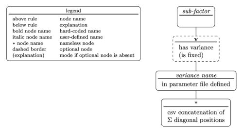
Sub-factor specifiers are used to communicate further information which may be that the sub-factor

• is a random sub-factor
• to which variance it is related to
• which diagonal element in the $$\Sigma$$ matrix of the variance it is related to

The tree diagram for the sub-factor specifier is

with the nested parentheses representation written as

sub-factor(v(variance name(diagonal position)))

According to the tree diagram the sub-factor specifier in the example model string translates to

• sub-factor name is u
• the sub-factor has a variance
• variance name is my_var
• the diagonal position in $$\Sigma$$ is #1.

Contrarily to variables, a sub-factor can have only one specifier assigned. That is, lmt would not accept a bi-variate model

y1=mu*b1+id*u1(v(myvar(1))
y2=mu*b2+id*u1(v(myvar(2))

because the two specifiers assigned to u1 , (v(myvar(1)) and (v(myvar(2) differ.